TDV-LeWM: Temporal-Difference Supervision for Latent World-Model Planning
Applying TDV-style motion learning to LeWM on OGBench-Cube
a) TDV-LeWM CEM Goal Completion Compared to LeWM
b) No Operation (no-op) Example
c) MPC CEM Success Rates and No-op Effects
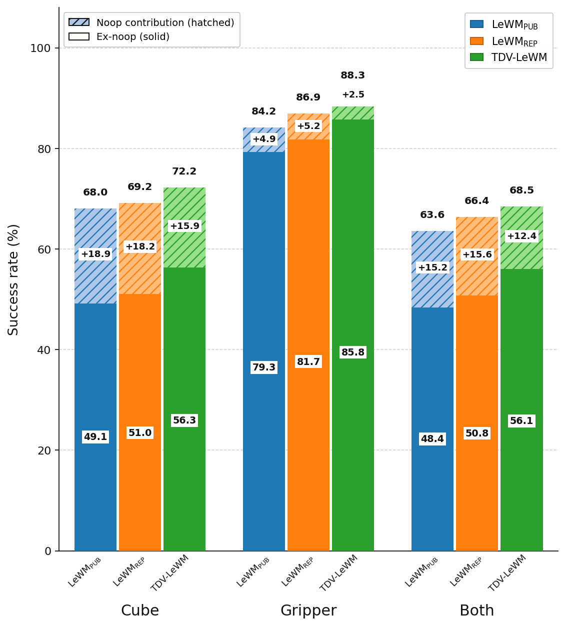
Joint-Embedding Predictive Architecture (JEPA) world models are becoming increasingly capable, with LeWM showing that a small, simple architecture using SIGReg can learn effective latent dynamics directly from pixels. Recent work on Temporal Difference in Vision (TDV) introduced a self-supervised learning signal based on the causal structure of pixel differences in video, with particular strength in visually dense environments. In this work, I add a TDV-style auxiliary representation-learning signal in the form of a transformer-based motion encoder to LeWM to bias its representation away from appearance and toward motion and task-relevant geometry. I train the model end-to-end on a single GPU and evaluate it on OGBench-Cube, the most visually complex task studied by LeWM and its weakest-performing benchmark. I also find that roughly 38% of OGBench-Cube evaluation scenarios are already successful at initialization, inflating reported performance. On the remaining non-trivial scenarios, LeWM achieves only about 50% cube success, while TDV-LeWM reaches 56%, a 5.3 percentage-point improvement across 15k scenarios. Because LeWM optimizes the latent representation of the full image, I also evaluate gripper and joint cube-gripper outcomes, where the TDV inductive bias improves performance consistently and the gains generally widen after removing no-operation cases.
Overview
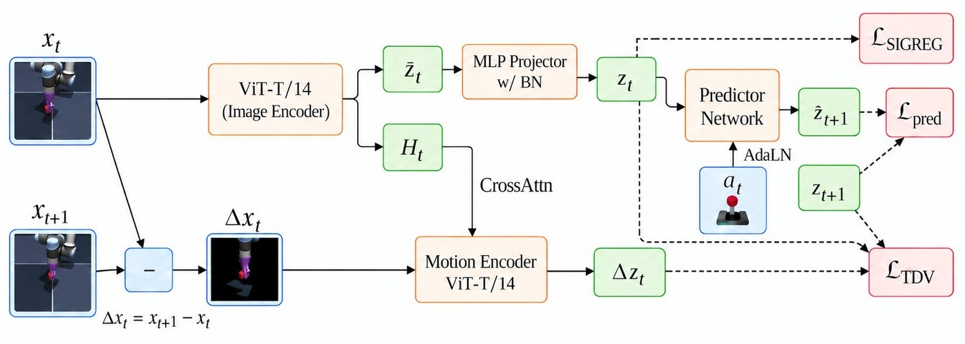
- Architecture. I augment LeWM with a motion encoder and a TDV-style temporal prediction loss. The motion encoder \(m_\phi\) takes the pixel difference \(\Delta x_t\) and cross-attends to the current latent feature map \(H_t\), producing a latent displacement \(\Delta z_t\). This displacement is trained such that \(z_t+\Delta z_t\approx z_{t+1}\).
- Collapse prevention. I kept LeWM’s SIGReg term and did not retrain TDV’s DINO-style teacher network with a stop-gradient (redundant with SIGReg regularization).
- Motion encoder \(m_\phi\). \(\Delta x_t = x_{t+1} - x_t\) is patchified and fed to a ViT-T/14 motion encoder that cross-attends to the image encoder’s feature map \(H_t\). \(\Delta z_t\) is outputted from the CLS token. The TDV paper found that contextualizing pixel differences with the current latent was important.
- Data. OGBench-Cube (single cube) through stable-worldmodel (SWM) (galilai-group/ogb_cube_single). I kept the usual frameskip of 5 and scenario horizon of 25.
- No-op Analysis. A no-op is a scenario whose start displacement is already below the 0.04 success threshold. In the OGBench-Cube sampling used by stable-worldmodel, about 38% of eval scenarios are cube no-ops (the object typically used for success rates), ~9% are gripper no-ops, and ~4% are both (union ~43%). These cases inflate reported success, especially cube and both-object metrics.
- Training. ViT-T/14 encoder, 10 epochs, batch size 128, learning rate \(5\times 10^{-5}\), on RTX 5090s via RunPod. Best TDV-LeWM run: \(\alpha=1.0\), \(\lambda=0.25\). My reproduction of LeWM, \(\mathrm{LeWM_{REP}}\), uses \(\lambda=0.1\).
- TDV-LeWM MPC Analysis. TDV-LeWM outperforms LeWM on every MPC planner (CEM, iCEM, and Adam); the gap is largest under CEM: both-object success 68.5% vs 66.4% / 63.6% for \(\mathrm{LeWM_{REP}}\) / \(\mathrm{LeWM_{PUB}}\), and 56.1% vs 50.8% / 48.4% with noops removed. TDV's benefit decreases with stronger planners such as iCEM.
- TDV-LeWM Planning Analysis. This analysis measured whether latent costs rank physically better action sequences. TDV-LeWM gives the best ranking of cube outcomes and the combined cube–gripper objective, with pooled Spearman correlations of \(\rho_{\mathrm{cube}} = 0.608\) and \(\rho_{\mathrm{cg}} = 0.657\), and positive \(\rho_{\mathrm{cg}}\) on 94% of scenarios. Across all models, gripper outcomes are ranked more faithfully than cube outcomes.
- Latent Straightening. Motivated by recent work on temporal straightening for planning in JEPA world models (Wang et al.), I analyzed whether TDV induces implicit temporal straightening of \(z_t\). TDV explicitly parameterizes the one-step latent displacement as \(z_{t+1}\approx z_t+\Delta z_t\), with the motion encoder directly learning the latent “velocity” \(z_{t+1}-z_t\). However, I found that TDV does not increase the paper’s straightness metric, \(C_t=\cos(z_{t+1}-z_t,\;z_{t+2}-z_{t+1})\), and therefore does not appear to reduce latent trajectory curvature.
Training dynamics
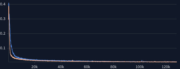
(a) Prediction loss \(\mathcal{L}_{\mathrm{pred}}\)
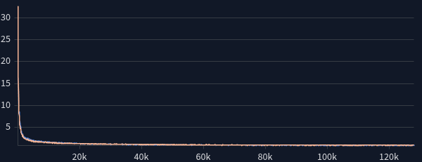
(b) SIGReg loss \(\mathcal{L}_{\mathrm{SIGReg}}\)
(c) TDV residual loss \(\mathcal{L}_{\mathrm{TDV}}\)
(d) Total loss \(\mathcal{L}\)
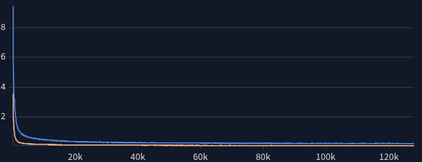
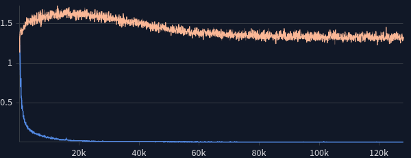
Loss curves for the terms in \(\mathcal{L}\). TDV-LeWM needed a larger SIGReg weight (\(\lambda=0.25\) vs \(0.1\)) to offset the extra predictive bias. Other SIGReg hyperparameters were left at the SWM library defaults (1024 projections, 17 knots). If we set \(\alpha=0\) in TDV-LeWM, then it is equivalent to vanilla LeWM, and we can still measure TDV's loss (before it is zeroed out in the loss by \(\alpha\)) via its motion encoder. This is visualized in c) and labeled as LeWM\(_{REP}\). We see that that as LeWM trains \(z_t\) becomes predictive of \(z_{t+1}\),reducing the TDV loss despite the noise from the untrained motion encoder.
Collapse Diagnostics
(a) Mean per-coordinate variance
(b) RMS of the embedding mean
(c) Roy–Vetterli effective rank (fraction of \(D\))
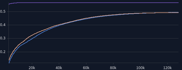
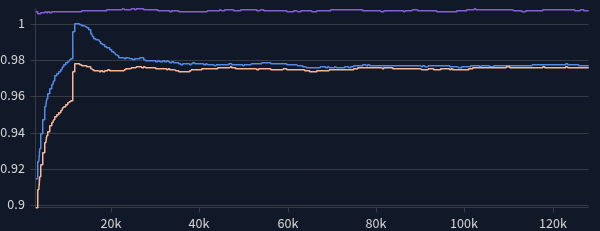
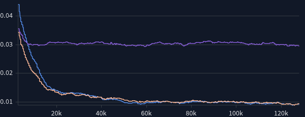
Collapse diagnostics on post-projection embeddings across optimization steps (over 10 epochs), with frozen \(\mathrm{LeWM_{PUB}}\) as a reference. The short transient in (b) and (c) for the frozen published model is the temporal averaging buffer filling up. \(\mathrm{LeWM_{PUB}}\) keeps a slightly higher Roy–Vetterli effective rank than both models I trained.
OGBench-Cube No-Operation Scenarios
A no-op is defined as a scenario whose start displacement is already below the 4cm success threshold for OGBench-Cube in the Mujoco simulator. Thereby, these scenarios are trivially successful for any planner. This occurs as a sampling artifact because the evaluation set samples random 25-step sequences from the dataset, and a large percentage of sequences have starting and ending object positions within the 4cm threshold. The table below shows the no-op counts for the cube, gripper, and both objects across 15k randomly sampled scenarios over 3 seeds
I include gripper no-ops because LeWM encodes the full scene into a single latent. As the next section shows, LeWM typically prioritizes minimizing gripper latent displacement over the cube's.
| Seed | Cube | Gripper | Both |
|---|---|---|---|
| 7 | 1850/5000 (37.0%) | 447/5000 (8.9%) | 190/5000 (3.8%) |
| 42 | 1957/5000 (39.1%) | 465/5000 (9.3%) | 221/5000 (4.4%) |
| 101 | 1899/5000 (38.0%) | 456/5000 (9.1%) | 214/5000 (4.3%) |
| Pooled | 5706/15000 (38.0%) | 1368/15000 (9.1%) | 625/15000 (4.2%) |
Cube no-ops make up ~38% of the evaluation set and account for most of the inflation in cube and both success rates. Gripper no-ops make up ~9%. The joint both-no-op rate is only ~4%, meaning that most cube no-ops still require the gripper to move. The union of scenarios where either the cube or gripper is already at goal is 6449/15000 (43.0%).
OGBench-Cube Retaining Discriminative Power Discussion
In a recent work, LpWM (Kuang et al., 2026), the authors write in the appendix under “Planning and Evaluation” (p. 15):
For OGBench-Cube, we follow the evaluation protocol of Maes et al. [2026b], where goal observations are sampled only 25 raw environment steps ahead. This short horizon can make the planning task relatively easy, potentially leading to performance saturation and limiting the discriminative power of the benchmark. We leave evaluation under more challenging longer-horizon and larger-frameskip settings to future work.
I argue that the apparent saturation of OGBench-Cube and the planning task appearing “easy” is not simply a consequence of short-horizon planning; the standard evaluation is heavily biased toward trivially successful configurations: 38% of episodes begin with the cube already inside the success threshold. Once these initially satisfied cases are removed, the apparent saturation, documented at 65–70% in Figure 4a of the LpWM paper, largely disappears and the benchmark retains discriminative power. More fundamentally, it is difficult to reconcile characterizing the planning problem as “easy” with reported success rates below 75% (in LeWM, LpWM, and across many other works), particularly when a substantial fraction of the evaluation set is already successful at initialization.
Evaluation: MPC Success Rates
Evaluation was done using the method in LeWM paper and the standard method for SWM on the OGBench-Cube task: anytime displacement of the cube below 4cm from its goal position. Because the latent represents the state of the entire image, I introduce two other metrics: the gripper's goal displacement, and "both", meaning the cube and gripper each reach their goal (the intersection of the two success events). For the gripper I use the same anytime goal displacement threshold of 4cm.
As discussed in the No-Op Evaluation section, the sampling distribution of OGBench-Cube includes a plethora of no-op scenarios for the cube and gripper. The following table shows the MPC success rates across various planners, including conditioning on removal of no-op scenarios.
| Planner | Model | Cube | Cube ex-noop | Grip | Grip ex-noop | Both | Both ex-noop |
|---|---|---|---|---|---|---|---|
| CEM | LeWMREP | 69.2% | 51.0% | 86.9% | 81.8% | 66.4% | 50.8% |
| LeWMPUB | 68.0% | 49.1% | 84.2% | 79.3% | 63.6% | 48.4% | |
| TDV-LeWM | 72.2% | 56.3% | 88.3% | 85.8% | 68.5% | 56.1% | |
| iCEM | LeWMREP | 69.8% | 51.9% | 83.1% | 76.7% | 65.7% | 51.6% |
| LeWMPUB | 71.7% | 54.1% | 78.5% | 74.5% | 63.9% | 53.2% | |
| TDV-LeWM | 73.7% | 57.6% | 83.2% | 80.4% | 67.2% | 56.6% | |
| Adam | LeWMREP | 68.7% | 48.6% | 79.2% | 70.6% | 64.0% | 48.2% |
| LeWMPUB | 69.1% | 49.3% | 77.1% | 67.8% | 63.6% | 48.1% | |
| TDV-LeWM | 70.5% | 51.8% | 81.7% | 76.1% | 65.1% | 51.0% |
CEM: \(n=15000\) (8551 ex-noop). iCEM and Adam: \(n=6000\) (3343 ex-noop). Pooled across seeds 7, 42, and 101.
TDV-LeWM performs the best with every planner, and the gap widens after removing no-ops, especially for cube/both (CEM both: +2.1 / +4.9 vs \(\mathrm{LeWM_{REP}}\) all / ex-noop). The performance benefit of TDV decreases with a more powerful planner (iCEM and Adam). All three models optimize gripper displacement more effectively than cube displacement, consistent with the gripper occupying a larger share of the image and therefore having greater influence in the latent representation.
Evaluation: Latent Cost Ranking
As an additional evaluation, I measure whether the latent cost used by MPC correctly ranks candidate action sequences by their true physical outcomes, an important property for effective MPC.
For a fixed initial state and goal, I sample candidate action sequences \((a^{(1)},\dots,a^{(N)})\). For each candidate, the world model predicts the terminal latent
with latent planning cost
The same action sequence is then executed in the simulator to measure the resulting physical costs:
I also define a normalized combined cost
I then compute the Spearman rank correlations
Higher positive \(\rho\) means that action sequences preferred by the latent objective also tend to produce better physical outcomes, which is the ranking behavior useful for MPC.
Pooled over 3 seeds, 600 scenarios \(\times\) 64 candidates. mean\(\pm\)std is per-scenario \(\rho\); parentheses are pooled \(\rho\).
| Model | \(\rho_{\mathrm{cube}}\) | \(\rho_{\mathrm{grip}}\) | \(\rho_{\mathrm{cg}}\) | %\(\rho>0\) cg |
|---|---|---|---|---|
| LeWMREP | +0.135±0.212 (+0.563) | +0.444±0.296 (+0.514) | +0.417±0.277 (+0.632) | 90% |
| LeWMPUB | +0.136±0.211 (+0.596) | +0.396±0.282 (+0.485) | +0.386±0.255 (+0.638) | 92% |
| TDV-LeWM | +0.165±0.199 (+0.608) | +0.431±0.262 (+0.521) | +0.426±0.230 (+0.657) | 94% |
TDV-LeWM gives the strongest ranking of cube outcomes and the combined objective, while all three models rank gripper outcomes substantially more faithfully than cube outcomes.
Latent Straightening
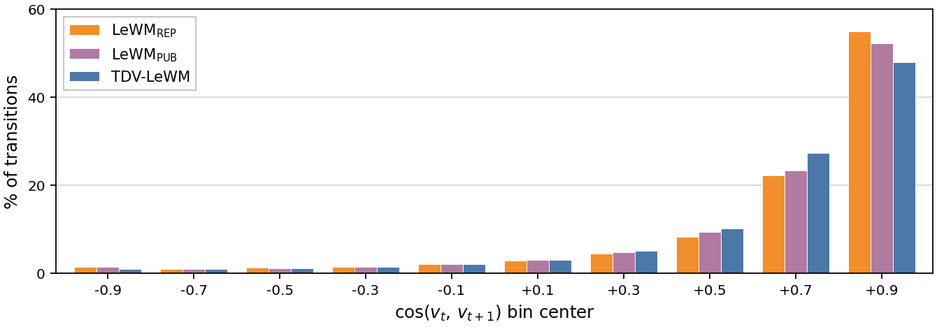
Motivated by recent work on temporal straightening for planning in JEPA world models (Wang et al.), I analyzed whether TDV induces implicit temporal straightening of \(z_t\). In the paper, Wang et al. define a latent trajectory as locally straight when consecutive velocities \(v_t = z_{t+1}-z_t\) and \(v_{t+1}=z_{t+2}-z_{t+1}\) point in similar directions as measured by their cosine similarity.
Larger values of \(C_t\) indicate that consecutive latent velocities are more aligned, corresponding to a locally straighter latent trajectory.
TDV explicitly parameterizes the one-step latent displacement as \(z_{t+1}\approx z_t+\Delta z_t\), with the motion encoder directly learning the latent “velocity” \(z_{t+1}-z_t\). This raisesed the question of whether TDV might implicitly encourage temporal straightening within the latent trajectory.
| Model | Mean | Std |
|---|---|---|
| LeWMREP | +0.674 | 0.382 |
| LeWMPUB | +0.669 | 0.381 |
| TDV-LeWM | +0.661 | 0.358 |
TDV-LeWM has a slightly lower mean consecutive-velocity cosine similarity (\(0.661\)) than LeWMREP (\(0.674\)) and LeWMPUB (\(0.669\)). TDV also places fewer transitions in the highest-alignment bin, \([0.80,1.00]\): 47.9% vs. 54.9% and 52.3% for LeWM\(_\mathrm{REP}\) and LeWM\(_\mathrm{PUB}\); however, it has more transitions instead falling into \([0.60,0.80)\). Together with the approximately unchanged mean straightness score, this suggests that the TDV augmentation turns out to not introduce any noticeable effect on straightening the latent space.
Future work
- Action-ambiguous environments. TDV’s pixel-difference bias may provide larger gains in settings where actions do not fully explain visual transitions, such as Atari.
- Appearance robustness. Since TDV derives features from temporal differences rather than absolute appearance, it may improve robustness to color and texture shifts that substantially degrade LeWM. Stable-WorldModel’s Push-T robustness suite is able to directly a directly test this.
- Motion-encoder contextualization. The current \(m_\phi\) contextualizes \(\Delta x_t\) by cross-attending to the encoder feature map \(H_t\). An ablation would instead run self-attention over the pixel-difference tokens and condition on the projected embedding \(z_t\) via AdaLN, testing whether TDV needs the spatial feature map or whether a compact latent is sufficient context.
Infrastructure
Training and evaluation were primarily done on the Runpod Community cloud. I opted to build deployment infrastructure to quickly perform hyperparameter sweeps and run various evaluation types across different seeds. The infrastructure I built can be visualized in the figure on the right and was robust to Runpod's commonly unreliable NVIDIA drivers and occasional machine crashes.
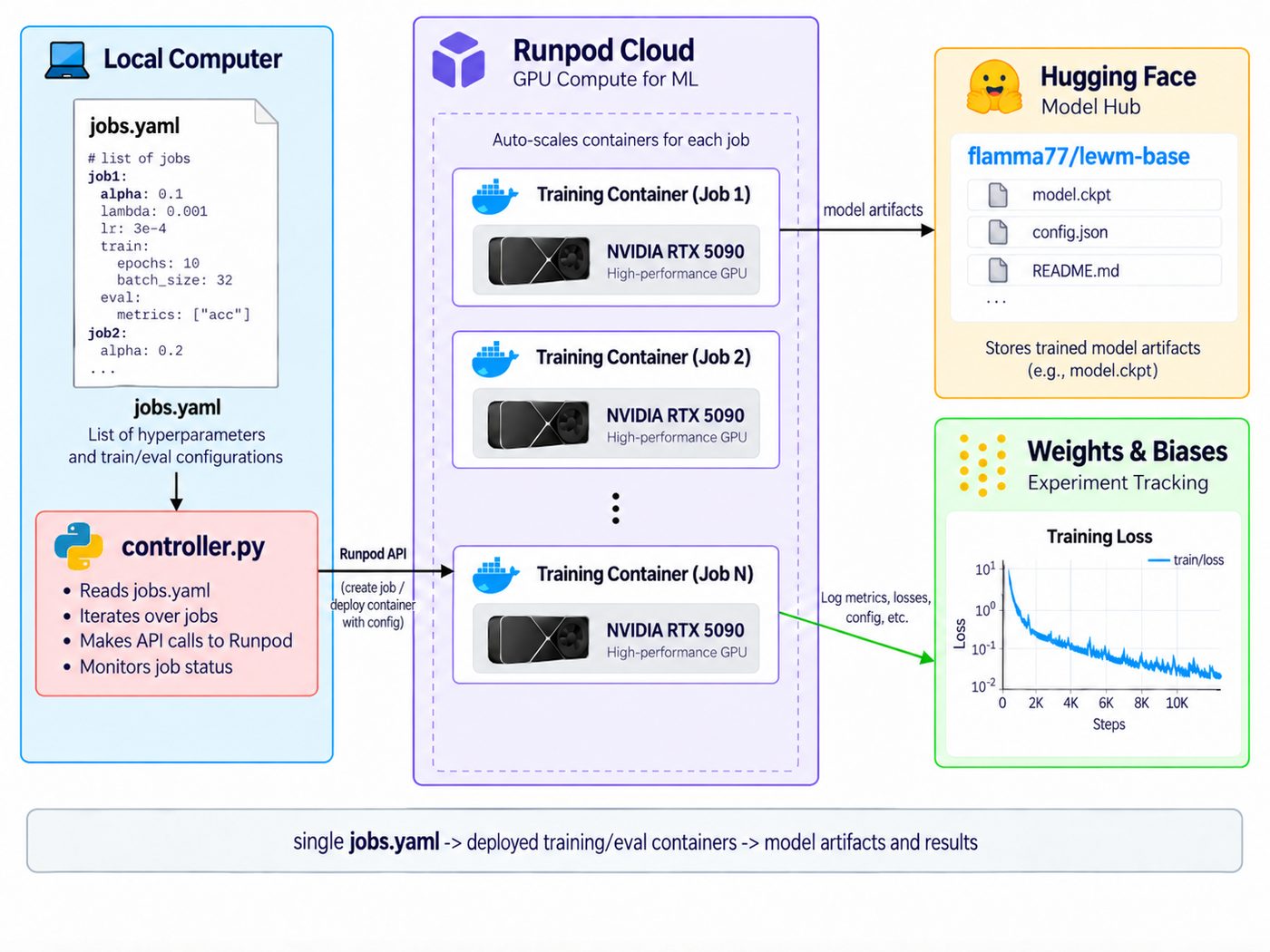
jobs.yaml drives training and eval containers on RunPod. Artifacts go to
Hugging Face;
metrics go to Weights & Biases. Failed driver detections recycle the pod onto another machine.
References
- Ninad Daithankar, Alexi Gladstone, Yann LeCun, and Heng Ji. You Don’t Need Strong Assumptions: Visual Representation Learning via Temporal Differences. arXiv, 2026. arXiv:2606.15956
- Lucas Maes, Quentin Le Lidec, Damien Scieur, Yann LeCun, and Randall Balestriero. LeWorldModel: Stable End-to-End Joint-Embedding Predictive Architecture from Pixels. arXiv, 2026. arXiv:2603.19312
- Yilun Kuang, Yash Dagade, Quentin Le Lidec, Lucas Maes, Randall Balestriero, and Yann LeCun. LpWM: A Case for Sparse Representations in World Models. arXiv, 2026. arXiv:2608.22764
- Randall Balestriero and Yann LeCun. LeJEPA: Provable and Scalable Self-Supervised Learning Without the Heuristics. arXiv, 2025. arXiv:2511.08544
- Seohong Park, Kevin Frans, Benjamin Eysenbach, and Sergey Levine. OGBench: Benchmarking Offline Goal-Conditioned RL. ICLR, 2025. arXiv:2410.20092
- Ying Wang, Oumayma Bounou, Gaoyue Zhou, Randall Balestriero, Tim G. J. Rudner, Yann LeCun, and Mengye Ren. Temporal Straightening for Latent Planning. arXiv, 2026. arXiv:2603.12231